Protein Ligand Complex MD Setup tutorial using BioExcel Building Blocks (biobb)

Based on the official Gromacs tutorial: http://www.mdtutorials.com/gmx/complex/index.html

This tutorial aims to illustrate the process of setting up a simulation system containing a protein in complex with a ligand, step by step, using the BioExcel Building Blocks library (biobb). The particular example used is the T4 lysozyme L99A/M102Q protein (PDB code 3HTB, https://doi.org/10.2210/pdb3HTB/pdb), in complex with the 2-propylphenol small molecule (3-letter Code JZ4, https://www.rcsb.org/ligand/JZ4).

Settings

Biobb modules used

biobb_io: Tools to fetch biomolecular data from public databases.
biobb_model: Tools to model macromolecular structures.
biobb_chemistry: Tools to manipulate chemical data.
biobb_gromacs: Tools to setup and run Molecular Dynamics simulations.
biobb_analysis: Tools to analyse Molecular Dynamics trajectories.
biobb_structure_utils: Tools to modify or extract information from a PDB structure file.

Auxiliary libraries used

jupyter: Free software, open standards, and web services for interactive computing across all programming languages.
nglview: Jupyter/IPython widget to interactively view molecular structures and trajectories in notebooks.
plotly: Python interactive graphing library integrated in Jupyter notebooks.
simpletraj: Lightweight coordinate-only trajectory reader based on code from GROMACS, MDAnalysis and VMD.

Conda Installation and Launch

git clone https://github.com/bioexcel/biobb_wf_protein-complex_md_setup.git
cd biobb_wf_protein-complex_md_setup
conda env create -f conda_env/environment.yml
conda activate biobb_Protein-Complex_MDsetup_tutorial
jupyter-notebook biobb_wf_protein-complex_md_setup/notebooks/biobb_Protein-Complex_MDsetup_tutorial.ipynb

Input parameters

Input parameters needed:

pdbCode: PDB code of the protein-ligand complex structure (e.g. 3HTB, https://doi.org/10.2210/pdb3HTB/pdb)
ligandCode: Small molecule 3-letter code for the ligand structure (e.g. JZ4, https://www.rcsb.org/ligand/JZ4)
mol_charge: Charge of the small molecule, needed to add hydrogen atoms.

import nglview
import ipywidgets
import os
import zipfile

pdbCode = "3HTB"
ligandCode = "JZ4"
mol_charge = 0

Fetching PDB structure

Downloading PDB structure with the protein-ligand complex from the RCSB PDB database.
Alternatively, a PDB file can be used as starting structure.
Splitting the molecule in three different files:

proteinFile: Protein structure
ligandFile: Ligand structure
complexFile: Protein-ligand complex structure

Building Blocks used:

Pdb from biobb_io.api.pdb

# Downloading desired PDB file 
# Import module
from biobb_io.api.pdb import pdb

# Create properties dict and inputs/outputs
downloaded_pdb = pdbCode+'.orig.pdb'
prop = {
    'pdb_code': pdbCode,
    'filter': False
}

# Create and launch bb
pdb(output_pdb_path=downloaded_pdb,
    properties=prop)

# Extracting Protein, Ligand and Protein-Ligand Complex to three different files
# Import module
from biobb_structure_utils.utils.extract_heteroatoms import extract_heteroatoms
from biobb_structure_utils.utils.extract_molecule import extract_molecule
from biobb_structure_utils.utils.cat_pdb import cat_pdb

# Create properties dict and inputs/outputs
proteinFile = pdbCode+'.pdb'
ligandFile = ligandCode+'.pdb'
complexFile = pdbCode+'_'+ligandCode+'.pdb'

prop = {
     'heteroatoms' : [{"name": "JZ4"}]
}

extract_heteroatoms(input_structure_path=downloaded_pdb,
     output_heteroatom_path=ligandFile,
     properties=prop)

extract_molecule(input_structure_path=downloaded_pdb,
     output_molecule_path=proteinFile)

print(proteinFile, ligandFile, complexFile)

cat_pdb(input_structure1=proteinFile,
       input_structure2=ligandFile,
       output_structure_path=complexFile)

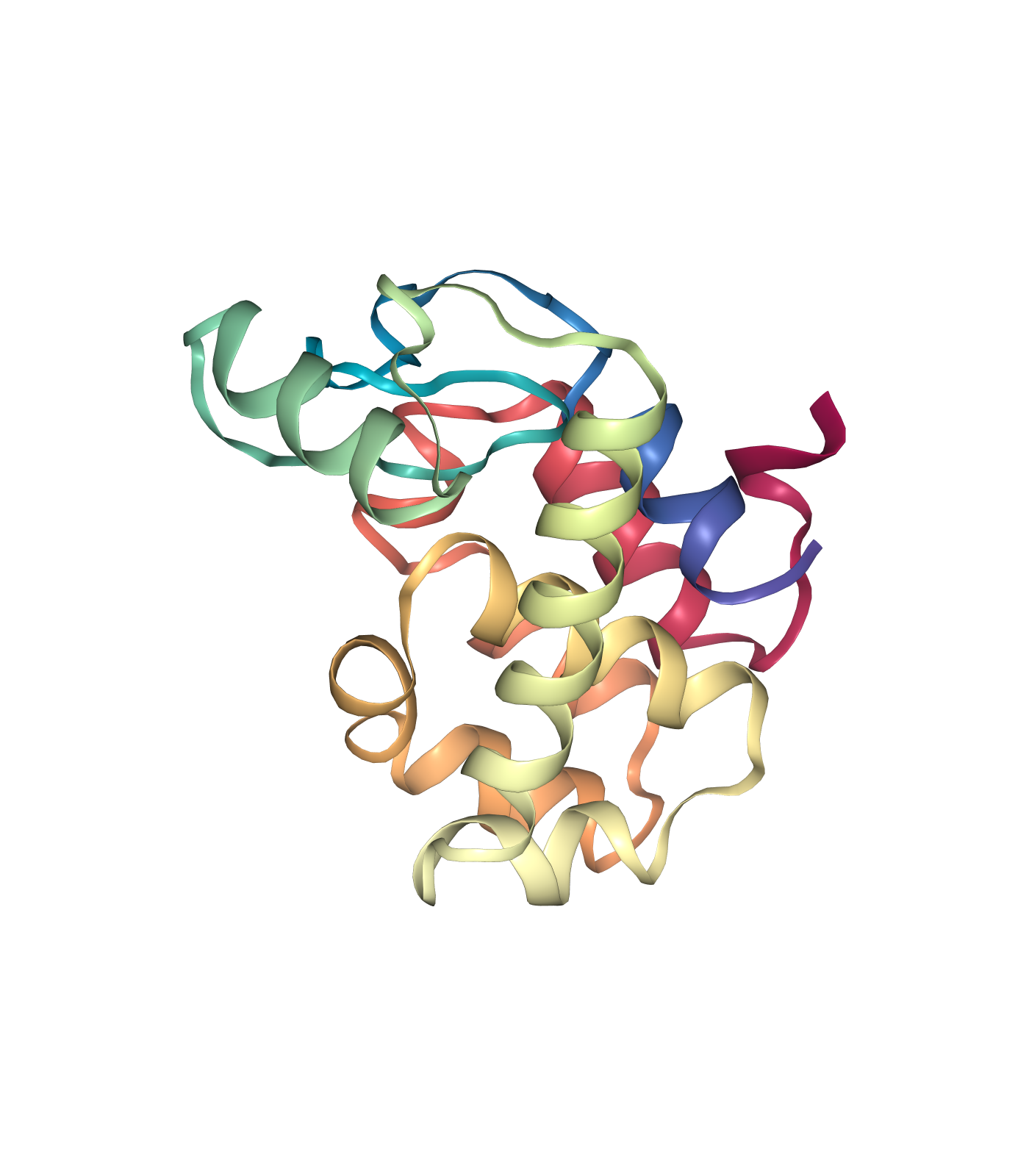
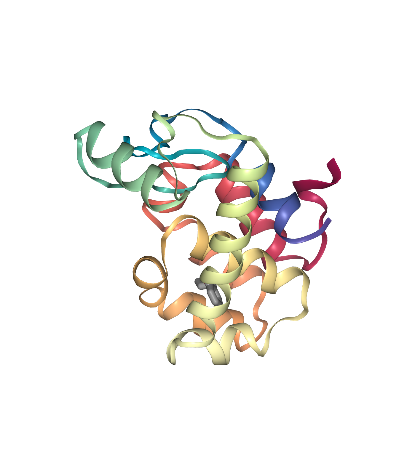
Visualizing 3D structures

Visualizing the generated PDB structures using NGL:

Protein structure (Left)
Ligand structure (Center)
Protein-ligand complex (Right)

# Show structures: protein, ligand and protein-ligand complex
view1 = nglview.show_structure_file(proteinFile)
view1._remote_call('setSize', target='Widget', args=['350px','400px'])
view1.camera='orthographic'
view1
view2 = nglview.show_structure_file(ligandFile)
view2.add_representation(repr_type='ball+stick')
view2._remote_call('setSize', target='Widget', args=['350px','400px'])
view2.camera='orthographic'
view2
view3 = nglview.show_structure_file(complexFile)
view3.add_representation(repr_type='licorice', radius='.5', selection=ligandCode)
view3._remote_call('setSize', target='Widget', args=['350px','400px'])
view3.camera='orthographic'
view3
ipywidgets.HBox([view1, view2, view3])

Fix protein structure

Checking and fixing (if needed) the protein structure:

Modeling missing side-chain atoms, modifying incorrect amide assignments, choosing alternative locations.
Checking for missing backbone atoms, heteroatoms, modified residues and possible atomic clashes.

Building Blocks used:

FixSideChain from biobb_model.model.fix_side_chain

# Check & Fix Protein Structure
# Import module
from biobb_model.model.fix_side_chain import fix_side_chain

# Create prop dict and inputs/outputs
fixed_pdb = pdbCode+'_fixed.pdb'

# Create and launch bb
fix_side_chain(input_pdb_path=proteinFile,
             output_pdb_path=fixed_pdb)

Create protein system topology

Building GROMACS topology corresponding to the protein structure.
Force field used in this tutorial is amber99sb-ildn: AMBER parm99 force field with corrections on backbone (sb) and side-chain torsion potentials (ildn). Water molecules type used in this tutorial is spc/e.
Adding hydrogen atoms if missing. Automatically identifying disulfide bridges.

Generating two output files:

GROMACS structure (gro file)
GROMACS topology ZIP compressed file containing:
- GROMACS topology top file (top file)
- GROMACS position restraint file/s (itp file/s)

Building Blocks used:

Pdb2gmx from biobb_gromacs.gromacs.pdb2gmx

# Create Protein system topology
# Import module
from biobb_gromacs.gromacs.pdb2gmx import pdb2gmx

# Create inputs/outputs
output_pdb2gmx_gro = pdbCode+'_pdb2gmx.gro'
output_pdb2gmx_top_zip = pdbCode+'_pdb2gmx_top.zip'
prop = {
    'force_field' : 'amber99sb-ildn',
    'water_type': 'spce'
}

# Create and launch bb
pdb2gmx(input_pdb_path=fixed_pdb,
        output_gro_path=output_pdb2gmx_gro,
        output_top_zip_path=output_pdb2gmx_top_zip,
        properties=prop)

Create ligand system topology

Building GROMACS topology corresponding to the ligand structure.
Force field used in this tutorial step is amberGAFF: General AMBER Force Field, designed for rational drug design.

Step 1: Add hydrogen atoms if missing.
Step 2: Energetically minimize the system with the new hydrogen atoms.
Step 3: Generate ligand topology (parameters).

Building Blocks used:

ReduceAddHydrogens from biobb_chemistry.ambertools.reduce_add_hydrogens
BabelMinimize from biobb_chemistry.babelm.babel_minimize
AcpypeParamsGMX from biobb_chemistry.acpype.acpype_params_gmx

Step 1: Add hydrogen atoms

# Create Ligand system topology, STEP 1
# Reduce_add_hydrogens: add Hydrogen atoms to a small molecule (using Reduce tool from Ambertools package)
# Import module
from biobb_chemistry.ambertools.reduce_add_hydrogens import reduce_add_hydrogens

# Create prop dict and inputs/outputs
output_reduce_h = ligandCode+'.reduce.H.pdb' 
prop = {
    'nuclear' : 'true'
}

# Create and launch bb
reduce_add_hydrogens(input_path=ligandFile,
                   output_path=output_reduce_h,
                   properties=prop)

Step 2: Energetically minimize the system with the new hydrogen atoms.

# Create Ligand system topology, STEP 2
# Babel_minimize: Structure energy minimization of a small molecule after being modified adding hydrogen atoms
# Import module
from biobb_chemistry.babelm.babel_minimize import babel_minimize

# Create prop dict and inputs/outputs
output_babel_min = ligandCode+'.H.min.mol2'                              
prop = {
    'method' : 'sd',
    'criteria' : '1e-10',
    'force_field' : 'GAFF'
}


# Create and launch bb
babel_minimize(input_path=output_reduce_h,
              output_path=output_babel_min,
              properties=prop)

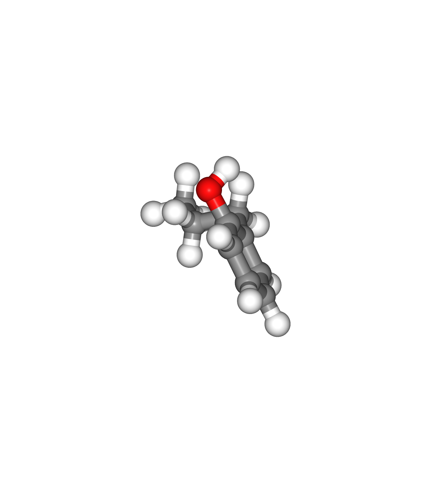
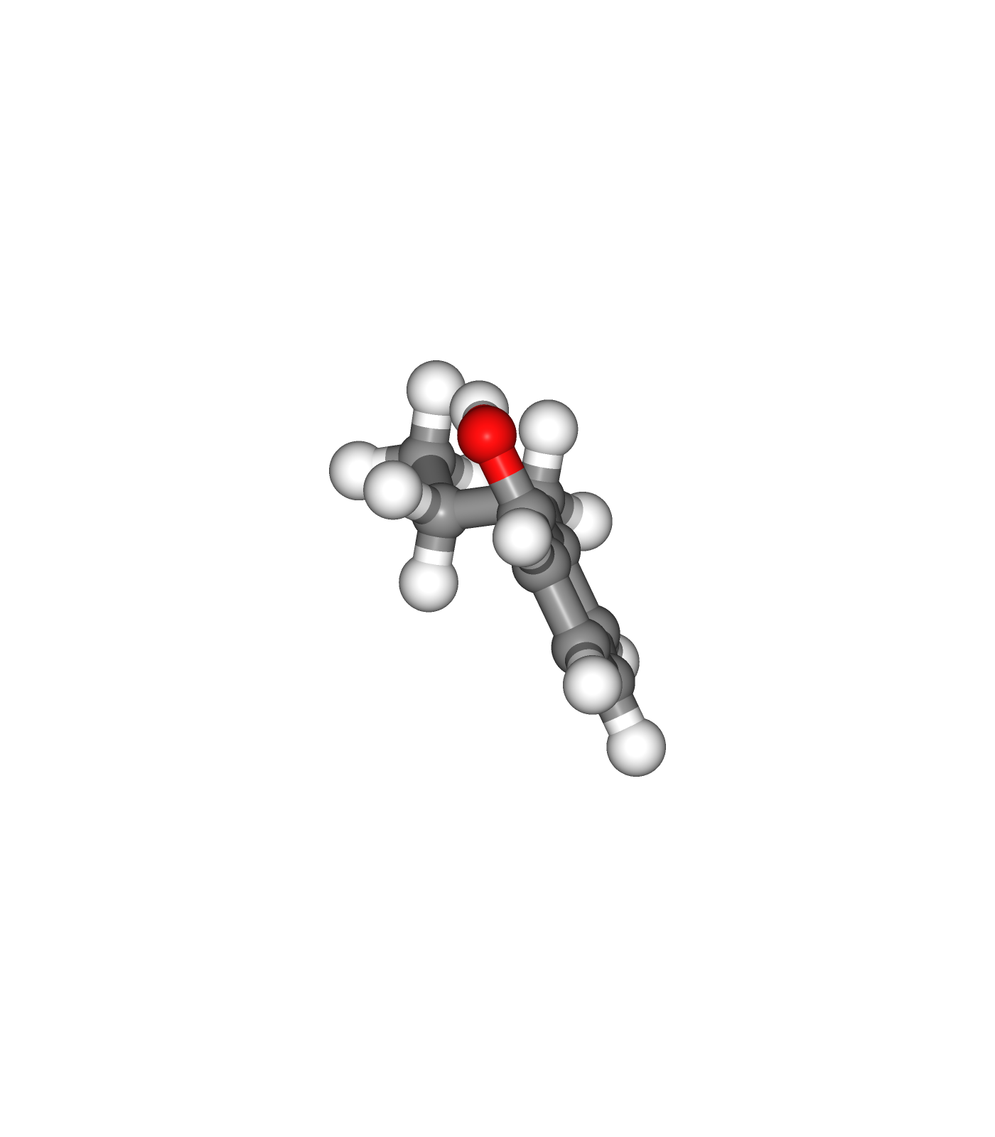
Visualizing 3D structures

Visualizing the small molecule generated PDB structures using NGL:

Original Ligand Structure (Left)
Ligand Structure with hydrogen atoms added (with Reduce program) (Center)
Ligand Structure with hydrogen atoms added (with Reduce program), energy minimized (with Open Babel) (Right)

# Show different structures generated (for comparison)

view1 = nglview.show_structure_file(ligandFile)
view1.add_representation(repr_type='ball+stick')
view1._remote_call('setSize', target='Widget', args=['350px','400px'])
view1.camera='orthographic'
view1
view2 = nglview.show_structure_file(output_reduce_h)
view2.add_representation(repr_type='ball+stick')
view2._remote_call('setSize', target='Widget', args=['350px','400px'])
view2.camera='orthographic'
view2
view3 = nglview.show_structure_file(output_babel_min)
view3.add_representation(repr_type='ball+stick')
view3._remote_call('setSize', target='Widget', args=['350px','400px'])
view3.camera='orthographic'
view3
ipywidgets.HBox([view1, view2, view3])

### Step 3: Generate ligand topology (parameters).

# Create Ligand system topology, STEP 3
# Acpype_params_gmx: Generation of topologies for GROMACS with ACPype
# Import module
from biobb_chemistry.acpype.acpype_params_gmx import acpype_params_gmx

# Create prop dict and inputs/outputs
output_acpype_gro = ligandCode+'params.gro'
output_acpype_itp = ligandCode+'params.itp'
output_acpype_top = ligandCode+'params.top'
output_acpype = ligandCode+'params'
prop = {
    'basename' : output_acpype,
    'charge' : mol_charge
}

# Create and launch bb
acpype_params_gmx(input_path=output_babel_min, 
                output_path_gro=output_acpype_gro,
                output_path_itp=output_acpype_itp,
                output_path_top=output_acpype_top,
                properties=prop)

Preparing Ligand Restraints

In subsequent steps of the pipeline, such as the equilibration stages of the protein-ligand complex system, it is recommended to apply some restraints to the small molecule, to avoid a possible change in position due to protein repulsion. Position restraints will be applied to the ligand, using a force constant of 1000 kJ/mol*nm^2 on the three coordinates: x, y and z. In this steps the restriction files will be created and integrated in the ligand topology.

Step 1: Creating an index file with a new group including just the small molecule heavy atoms.
Step 2: Generating the position restraints file.

Building Blocks used:

MakeNdx from biobb_gromacs.gromacs.make_ndx
Genrestr from biobb_gromacs.gromacs.genrestr

Step 1: Creating an index file for the small molecule heavy atoms

# MakeNdx: Creating index file with a new group (small molecule heavy atoms)
from biobb_gromacs.gromacs.make_ndx import make_ndx

# Create prop dict and inputs/outputs
output_ligand_ndx = ligandCode+'_index.ndx'
prop = {
    'selection': "0 & ! a H*"
}

# Create and launch bb
make_ndx(input_structure_path=output_acpype_gro,
        output_ndx_path=output_ligand_ndx,
        properties=prop)

Step 2: Generating the position restraints file

# Genrestr: Generating the position restraints file
from biobb_gromacs.gromacs.genrestr import genrestr

# Create prop dict and inputs/outputs
output_restraints_top = ligandCode+'_posres.itp'
prop = {
    'force_constants': "1000 1000 1000",
    'restrained_group': "System"
}

# Create and launch bb
genrestr(input_structure_path=output_acpype_gro,
         input_ndx_path=output_ligand_ndx,
         output_itp_path=output_restraints_top,
         properties=prop)

Create new protein-ligand complex structure file

Building new protein-ligand complex PDB file with:

The new protein system with fixed problems from Fix Protein Structure step and hydrogens atoms added from Create Protein System Topology step.
The new ligand system with hydrogens atoms added from Create Ligand System Topology step.

This new structure is needed for GROMACS as it is force field-compliant, it has all the new hydrogen atoms, and the atom names are matching the newly generated protein and ligand topologies.

Building Blocks used:

GMXTrjConvStr from biobb_analysis.gromacs.gmx_trjconv_str

# biobb analysis module
from biobb_analysis.gromacs.gmx_trjconv_str import gmx_trjconv_str
from biobb_structure_utils.utils.cat_pdb import cat_pdb

# Convert gro (with hydrogens) to pdb (PROTEIN)
proteinFile_H = pdbCode+'_'+ligandCode+'_complex_H.pdb'
prop = {
    'selection' : 'System'
}

# Create and launch bb
gmx_trjconv_str(input_structure_path=output_pdb2gmx_gro,
              input_top_path=output_pdb2gmx_gro,
              output_str_path=proteinFile_H, 
              properties=prop)

# Convert gro (with hydrogens) to pdb (LIGAND)
ligandFile_H = ligandCode+'_complex_H.pdb'
prop = {
    'selection' : 'System'
}

# Create and launch bb
gmx_trjconv_str(input_structure_path=output_acpype_gro,
              input_top_path=output_acpype_gro,
              output_str_path=ligandFile_H, 
              properties=prop)


# Concatenating both PDB files: Protein + Ligand
complexFile_H = pdbCode+'_'+ligandCode+'_H.pdb'

# Create and launch bb
cat_pdb(input_structure1=proteinFile_H,
       input_structure2=ligandFile_H,
       output_structure_path=complexFile_H)

Create new protein-ligand complex topology file

Building new protein-ligand complex GROMACS topology file with:

The new protein system topology generated from Create Protein System Topology step.
The new ligand system topology generated from Create Ligand System Topology step.

NOTE: From this point on, the protein-ligand complex structure and topology generated can be used in a regular MD setup.

Building Blocks used:

AppendLigand from biobb_gromacs.gromacs_extra.append_ligand (NOTE: link should be updated with the documentation)

# AppendLigand: Append a ligand to a GROMACS topology
# Import module
from biobb_gromacs.gromacs_extra.append_ligand import append_ligand

# Create prop dict and inputs/outputs
output_complex_top = pdbCode+'_'+ligandCode+'_complex.top.zip'

posresifdef = "POSRES_"+ligandCode.upper()
prop = {
    'posres_name': posresifdef
}

# Create and launch bb
append_ligand(input_top_zip_path=output_pdb2gmx_top_zip,
             input_posres_itp_path=output_restraints_top,
             input_itp_path=output_acpype_itp, 
             output_top_zip_path=output_complex_top,
             properties=prop)

Create solvent box

Define the unit cell for the protein-ligand complex to fill it with water molecules.
Truncated octahedron box is used for the unit cell. This box type is the one which best reflects the geometry of the solute/protein, in this case a globular protein, as it approximates a sphere. It is also convenient for the computational point of view, as it accumulates less water molecules at the corners, reducing the final number of water molecules in the system and making the simulation run faster.
A protein to box distance of 0.8 nm is used, and the protein is centered in the box.

Building Blocks used:

Editconf from biobb_gromacs.gromacs.editconf

# Editconf: Create solvent box
# Import module
from biobb_gromacs.gromacs.editconf import editconf

# Create prop dict and inputs/outputs
output_editconf_gro = pdbCode+'_'+ligandCode+'_complex_editconf.gro'

prop = {
    'box_type': 'octahedron',
    'distance_to_molecule': 0.8
}

# Create and launch bb
editconf(input_gro_path=complexFile_H, 
         output_gro_path=output_editconf_gro,
         properties=prop)

Fill the box with water molecules

Fill the unit cell for the protein-ligand complex with water molecules.
The solvent type used is the default Simple Point Charge water (SPC), a generic equilibrated 3-point solvent model.

Building Blocks used:

Solvate from biobb_gromacs.gromacs.solvate

# Solvate: Fill the box with water molecules
from biobb_gromacs.gromacs.solvate import solvate

# Create prop dict and inputs/outputs
output_solvate_gro = pdbCode+'_'+ligandCode+'_solvate.gro'
output_solvate_top_zip = pdbCode+'_'+ligandCode+'_solvate_top.zip'

# Create and launch bb
solvate(input_solute_gro_path=output_editconf_gro,
        output_gro_path=output_solvate_gro,
        input_top_zip_path=output_complex_top,
        output_top_zip_path=output_solvate_top_zip)

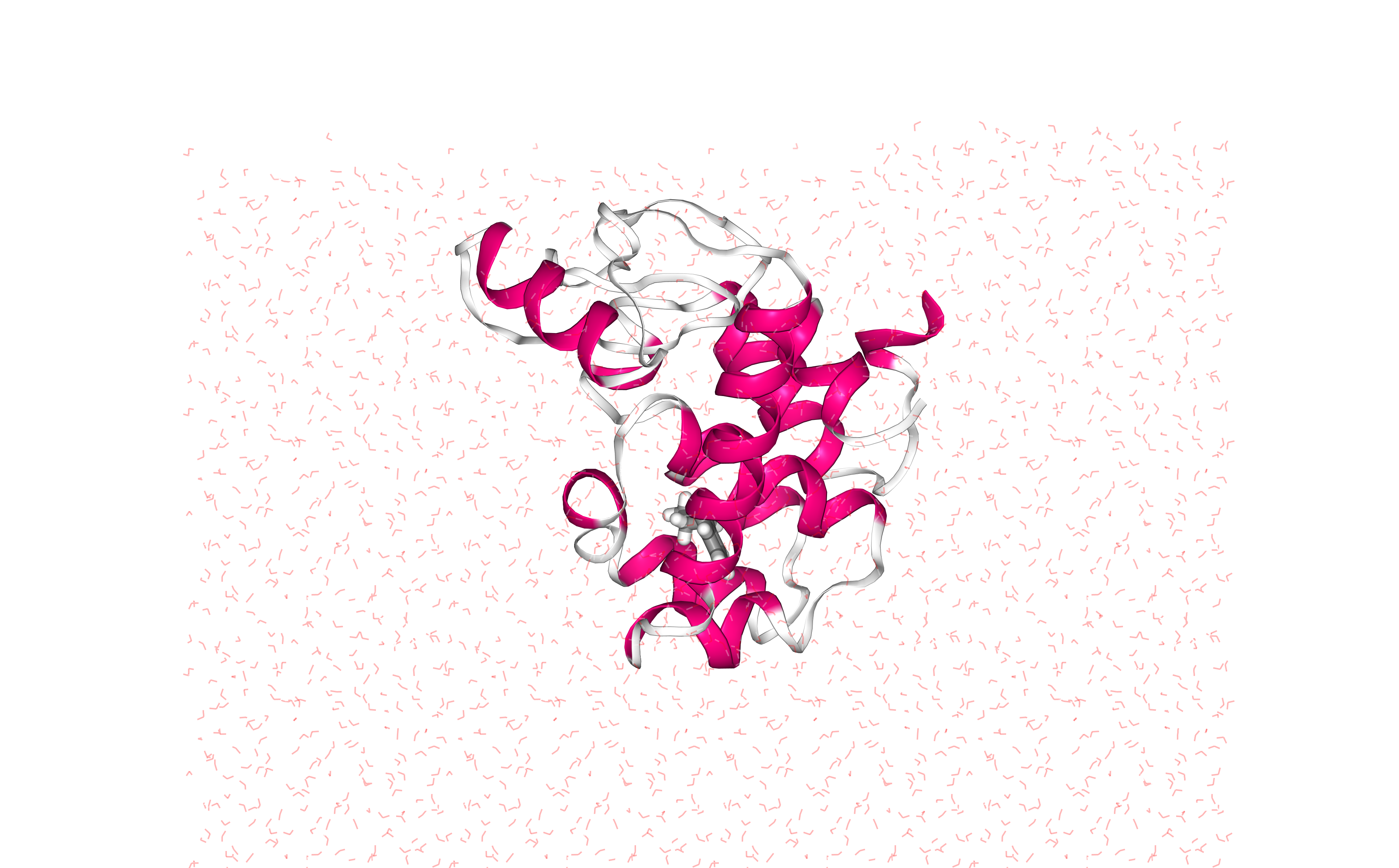
Visualizing 3D structure

Visualizing the protein-ligand complex with the newly added solvent box using NGL
Note the octahedral box filled with water molecules surrounding the protein structure, which is centered right in the middle of the box.

#Show protein
view = nglview.show_structure_file(output_solvate_gro)
view.clear_representations()
view.add_representation(repr_type='cartoon', selection='protein', color='sstruc')
view.add_representation(repr_type='licorice', radius='.5', selection=ligandCode)
view.add_representation(repr_type='line', linewidth='1', selection='SOL', opacity='.3')
view._remote_call('setSize', target='Widget', args=['','600px'])
view.camera='orthographic'
view

Adding ions

Add ions to neutralize the protein-ligand complex and reach a desired ionic concentration.

Step 1: Creating portable binary run file for ion generation
Step 2: Adding ions to neutralize the system and reach a 0.05 molar ionic concentration

Building Blocks used:

Grompp from biobb_gromacs.gromacs.grompp
Genion from biobb_gromacs.gromacs.genion

Step 1: Creating portable binary run file for ion generation

# Grompp: Creating portable binary run file for ion generation
from biobb_gromacs.gromacs.grompp import grompp

# Create prop dict and inputs/outputs
prop = {
    'mdp':{
        'nsteps':'5000'
    },
    'simulation_type':'minimization',
    'maxwarn': 1
}
output_gppion_tpr = pdbCode+'_'+ligandCode+'_complex_gppion.tpr'

# Create and launch bb
grompp(input_gro_path=output_solvate_gro,
       input_top_zip_path=output_solvate_top_zip, 
       output_tpr_path=output_gppion_tpr,
       properties=prop)

Step 2: Adding ions to neutralize the system and reach a 0.05 molar concentration

Replace solvent molecules with ions to neutralize the system and reaching a 0.05 molar ionic concentration

# Genion: Adding ions to reach a 0.05 molar concentration
from biobb_gromacs.gromacs.genion import genion

# Create prop dict and inputs/outputs
prop={
    'neutral':True,
    'concentration':0.05
}
output_genion_gro = pdbCode+'_'+ligandCode+'_genion.gro'
output_genion_top_zip = pdbCode+'_'+ligandCode+'_genion_top.zip'

# Create and launch bb
genion(input_tpr_path=output_gppion_tpr,
       output_gro_path=output_genion_gro, 
       input_top_zip_path=output_solvate_top_zip,
       output_top_zip_path=output_genion_top_zip, 
       properties=prop)

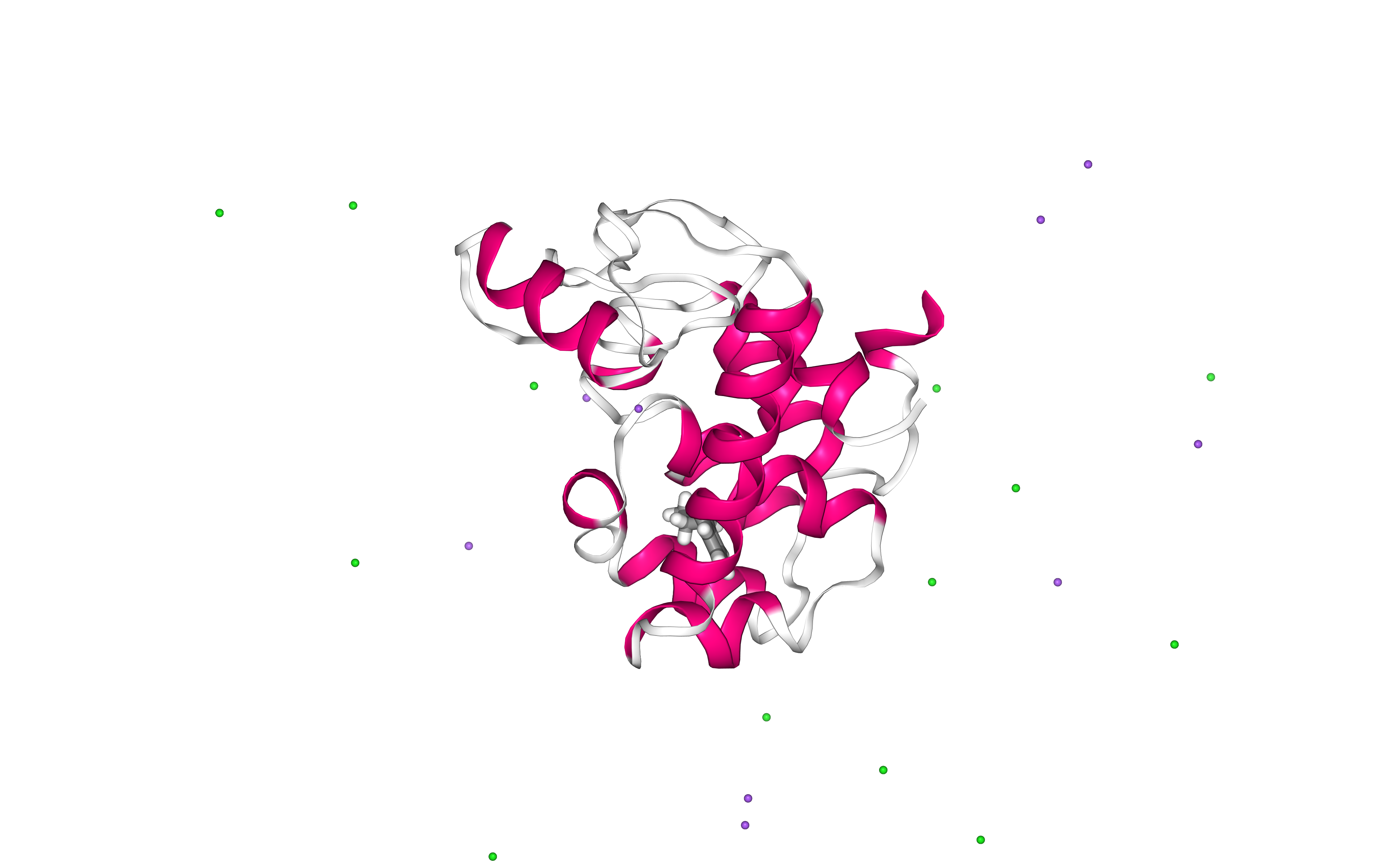
Visualizing 3D structure

Visualizing the protein-ligand complex with the newly added ionic concentration using NGL

#Show protein
view = nglview.show_structure_file(output_genion_gro)
view.clear_representations()
view.add_representation(repr_type='cartoon', selection='protein', color='sstruc')
view.add_representation(repr_type='licorice', radius='.5', selection=ligandCode)
view.add_representation(repr_type='ball+stick', selection='NA')
view.add_representation(repr_type='ball+stick', selection='CL')
view._remote_call('setSize', target='Widget', args=['','600px'])
view.camera='orthographic'
view

Energetically minimize the system

Energetically minimize the protein-ligand complex till reaching a desired potential energy.

Step 1: Creating portable binary run file for energy minimization
Step 2: Energetically minimize the protein-ligand complex till reaching a force of 500 kJ/mol*nm.
Step 3: Checking energy minimization results. Plotting energy by time during the minimization process.

Building Blocks used:

Grompp from biobb_gromacs.gromacs.grompp
Mdrun from biobb_gromacs.gromacs.mdrun
GMXEnergy from biobb_analysis.gromacs.gmx_energy

Step 1: Creating portable binary run file for energy minimization

Method used to run the energy minimization is a steepest descent, with a maximum force of 500 kJ/mol*nm^2, and a minimization step size of 1fs. The maximum number of steps to perform if the maximum force is not reached is 5,000 steps.

# Grompp: Creating portable binary run file for mdrun
from biobb_gromacs.gromacs.grompp import grompp

# Create prop dict and inputs/outputs
prop = {
    'mdp':{
        'nsteps':'5000',
        'emstep': 0.01,
        'emtol':'500'
    },
    'simulation_type':'minimization'
}
output_gppmin_tpr = pdbCode+'_'+ligandCode+'_gppmin.tpr'

# Create and launch bb
grompp(input_gro_path=output_genion_gro,
       input_top_zip_path=output_genion_top_zip,
       output_tpr_path=output_gppmin_tpr,
       properties=prop)

Step 2: Running Energy Minimization

Running energy minimization using the tpr file generated in the previous step.

# Mdrun: Running minimization
from biobb_gromacs.gromacs.mdrun import mdrun

# Create prop dict and inputs/outputs
output_min_trr = pdbCode+'_'+ligandCode+'_min.trr'
output_min_gro = pdbCode+'_'+ligandCode+'_min.gro'
output_min_edr = pdbCode+'_'+ligandCode+'_min.edr'
output_min_log = pdbCode+'_'+ligandCode+'_min.log'

# Create and launch bb
mdrun(input_tpr_path=output_gppmin_tpr,
      output_trr_path=output_min_trr, 
      output_gro_path=output_min_gro,
      output_edr_path=output_min_edr, 
      output_log_path=output_min_log)

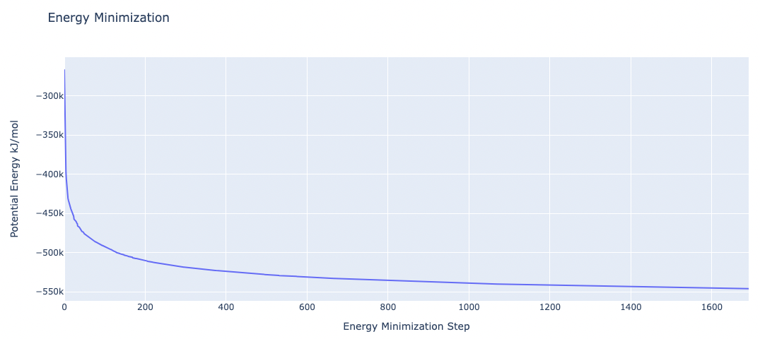
Step 3: Checking Energy Minimization results

Checking energy minimization results. Plotting potential energy by time during the minimization process.

# GMXEnergy: Getting system energy by time  
from biobb_analysis.gromacs.gmx_energy import gmx_energy

# Create prop dict and inputs/outputs
output_min_ene_xvg = pdbCode+'_'+ligandCode+'_min_ene.xvg'
prop = {
    'terms':  ["Potential"]
}

# Create and launch bb
gmx_energy(input_energy_path=output_min_edr, 
          output_xvg_path=output_min_ene_xvg, 
          properties=prop)

import plotly
import plotly.graph_objs as go

#Read data from file and filter energy values higher than 1000 kJ/mol
with open(output_min_ene_xvg,'r') as energy_file:
    x,y = map(
        list,
        zip(*[
            (float(line.split()[0]),float(line.split()[1]))
            for line in energy_file 
            if not line.startswith(("#","@")) 
            if float(line.split()[1]) < 1000 
        ])
    )

plotly.offline.init_notebook_mode(connected=True)

fig = ({
    "data": [go.Scatter(x=x, y=y)],
    "layout": go.Layout(title="Energy Minimization",
                        xaxis=dict(title = "Energy Minimization Step"),
                        yaxis=dict(title = "Potential Energy kJ/mol")
                       )
})

plotly.offline.iplot(fig)

Equilibrate the system (NVT)

Equilibrate the protein-ligand complex system in NVT ensemble (constant Number of particles, Volume and Temperature). To avoid temperature coupling problems, a new “system” group will be created including the protein + the ligand to be assigned to a single thermostatting group.

Step 1: Creating an index file with a new group including the protein-ligand complex.
Step 2: Creating portable binary run file for system equilibration
Step 3: Equilibrate the protein-ligand complex with NVT ensemble.
Step 4: Checking NVT Equilibration results. Plotting system temperature by time during the NVT equilibration process.

Building Blocks used:

MakeNdx from biobb_gromacs.gromacs.make_ndx
Grompp from biobb_gromacs.gromacs.grompp
Mdrun from biobb_gromacs.gromacs.mdrun
GMXEnergy from biobb_analysis.gromacs.gmx_energy

Step 1: Creating an index file with a new group including the protein-ligand complex

# MakeNdx: Creating index file with a new group (protein-ligand complex)
from biobb_gromacs.gromacs.make_ndx import make_ndx

# Create prop dict and inputs/outputs
output_complex_ndx = pdbCode+'_'+ligandCode+'_index.ndx'
prop = {
    'selection': "\"Protein\"|\"Other\"" 
}

# Create and launch bb
make_ndx(input_structure_path=output_min_gro,
        output_ndx_path=output_complex_ndx,
        properties=prop)

Step 2: Creating portable binary run file for system equilibration (NVT)

Note that for the purposes of temperature coupling, the protein-ligand complex (Protein_Other) is considered as a single entity.

# Grompp: Creating portable binary run file for NVT System Equilibration
from biobb_gromacs.gromacs.grompp import grompp

# Create prop dict and inputs/outputs
output_gppnvt_tpr = pdbCode+'_'+ligandCode+'gppnvt.tpr'
prop = {
    'mdp':{
        'nsteps':'5000',
        'tc-grps': 'Protein_Other Water_and_ions',
        'Define': '-DPOSRES -D' + posresifdef
    },
    'simulation_type':'nvt'
}

# Create and launch bb
grompp(input_gro_path=output_min_gro,
       input_top_zip_path=output_genion_top_zip,
       input_ndx_path=output_complex_ndx,
       output_tpr_path=output_gppnvt_tpr,
       properties=prop)

Step 3: Running NVT equilibration

# Mdrun: Running NVT System Equilibration 
from biobb_gromacs.gromacs.mdrun import mdrun

# Create prop dict and inputs/outputs
output_nvt_trr = pdbCode+'_'+ligandCode+'_nvt.trr'
output_nvt_gro = pdbCode+'_'+ligandCode+'_nvt.gro'
output_nvt_edr = pdbCode+'_'+ligandCode+'_nvt.edr'
output_nvt_log = pdbCode+'_'+ligandCode+'_nvt.log'
output_nvt_cpt = pdbCode+'_'+ligandCode+'_nvt.cpt'

# Create and launch bb
mdrun(input_tpr_path=output_gppnvt_tpr,
      output_trr_path=output_nvt_trr,
      output_gro_path=output_nvt_gro,
      output_edr_path=output_nvt_edr,
      output_log_path=output_nvt_log,
      output_cpt_path=output_nvt_cpt)

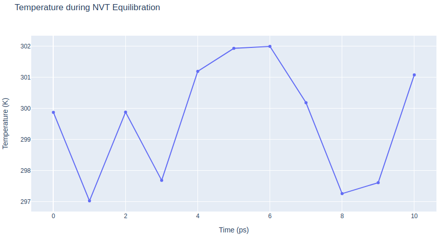
Step 4: Checking NVT Equilibration results

Checking NVT Equilibration results. Plotting system temperature by time during the NVT equilibration process.

# GMXEnergy: Getting system temperature by time during NVT Equilibration  
from biobb_analysis.gromacs.gmx_energy import gmx_energy

# Create prop dict and inputs/outputs
output_nvt_temp_xvg = pdbCode+'_'+ligandCode+'_nvt_temp.xvg'
prop = {
    'terms':  ["Temperature"]
}

# Create and launch bb
gmx_energy(input_energy_path=output_nvt_edr, 
          output_xvg_path=output_nvt_temp_xvg, 
          properties=prop)

import plotly
import plotly.graph_objs as go

# Read temperature data from file 
with open(output_nvt_temp_xvg,'r') as temperature_file:
    x,y = map(
        list,
        zip(*[
            (float(line.split()[0]),float(line.split()[1]))
            for line in temperature_file 
            if not line.startswith(("#","@")) 
        ])
    )

plotly.offline.init_notebook_mode(connected=True)

fig = ({
    "data": [go.Scatter(x=x, y=y)],
    "layout": go.Layout(title="Temperature during NVT Equilibration",
                        xaxis=dict(title = "Time (ps)"),
                        yaxis=dict(title = "Temperature (K)")
                       )
})

plotly.offline.iplot(fig)

Equilibrate the system (NPT)

Equilibrate the protein-ligand complex system in NPT ensemble (constant Number of particles, Pressure and Temperature) .

Step 1: Creating portable binary run file for system equilibration
Step 2: Equilibrate the protein-ligand complex with NPT ensemble.
Step 3: Checking NPT Equilibration results. Plotting system pressure and density by time during the NPT equilibration process.

Building Blocks used:

Grompp from biobb_gromacs.gromacs.grompp
Mdrun from biobb_gromacs.gromacs.mdrun
GMXEnergy from biobb_analysis.gromacs.gmx_energy

Step 1: Creating portable binary run file for system equilibration (NPT)

# Grompp: Creating portable binary run file for (NPT) System Equilibration
from biobb_gromacs.gromacs.grompp import grompp

# Create prop dict and inputs/outputs
output_gppnpt_tpr = pdbCode+'_'+ligandCode+'_gppnpt.tpr'
prop = {
    'mdp':{
        'type': 'npt',
        'nsteps':'5000',
        'tc-grps': 'Protein_Other Water_and_ions',
        'Define': '-DPOSRES -D' + posresifdef
    },
    'simulation_type':'npt'
}

# Create and launch bb
grompp(input_gro_path=output_nvt_gro,
       input_top_zip_path=output_genion_top_zip,
       input_ndx_path=output_complex_ndx,
       output_tpr_path=output_gppnpt_tpr,
       input_cpt_path=output_nvt_cpt,
       properties=prop)

Step 2: Running NPT equilibration

# Mdrun: Running NPT System Equilibration
from biobb_gromacs.gromacs.mdrun import mdrun

# Create prop dict and inputs/outputs
output_npt_trr = pdbCode+'_'+ligandCode+'_npt.trr'
output_npt_gro = pdbCode+'_'+ligandCode+'_npt.gro'
output_npt_edr = pdbCode+'_'+ligandCode+'_npt.edr'
output_npt_log = pdbCode+'_'+ligandCode+'_npt.log'
output_npt_cpt = pdbCode+'_'+ligandCode+'_npt.cpt'

# Create and launch bb
mdrun(input_tpr_path=output_gppnpt_tpr,
      output_trr_path=output_npt_trr,
      output_gro_path=output_npt_gro,
      output_edr_path=output_npt_edr,
      output_log_path=output_npt_log,
      output_cpt_path=output_npt_cpt)

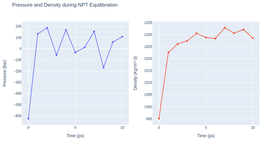
Step 3: Checking NPT Equilibration results

Checking NPT Equilibration results. Plotting system pressure and density by time during the NPT equilibration process.

# GMXEnergy: Getting system pressure and density by time during NPT Equilibration  
from biobb_analysis.gromacs.gmx_energy import gmx_energy

# Create prop dict and inputs/outputs
output_npt_pd_xvg = pdbCode+'_'+ligandCode+'_npt_PD.xvg'
prop = {
    'terms':  ["Pressure","Density"]
}

# Create and launch bb
gmx_energy(input_energy_path=output_npt_edr, 
          output_xvg_path=output_npt_pd_xvg, 
          properties=prop)

import plotly
from plotly import subplots
import plotly.graph_objs as go

# Read pressure and density data from file 
with open(output_npt_pd_xvg,'r') as pd_file:
    x,y,z = map(
        list,
        zip(*[
            (float(line.split()[0]),float(line.split()[1]),float(line.split()[2]))
            for line in pd_file 
            if not line.startswith(("#","@")) 
        ])
    )

plotly.offline.init_notebook_mode(connected=True)

trace1 = go.Scatter(
    x=x,y=y
)
trace2 = go.Scatter(
    x=x,y=z
)

fig = subplots.make_subplots(rows=1, cols=2, print_grid=False)

fig.append_trace(trace1, 1, 1)
fig.append_trace(trace2, 1, 2)

fig['layout']['xaxis1'].update(title='Time (ps)')
fig['layout']['xaxis2'].update(title='Time (ps)')
fig['layout']['yaxis1'].update(title='Pressure (bar)')
fig['layout']['yaxis2'].update(title='Density (Kg*m^-3)')

fig['layout'].update(title='Pressure and Density during NPT Equilibration')
fig['layout'].update(showlegend=False)

plotly.offline.iplot(fig)

Free Molecular Dynamics Simulation

Upon completion of the two equilibration phases (NVT and NPT), the system is now well-equilibrated at the desired temperature and pressure. The position restraints can now be released. The last step of the protein-ligand complex MD setup is a short, free MD simulation, to ensure the robustness of the system.

Step 1: Creating portable binary run file to run a free MD simulation.
Step 2: Run short MD simulation of the protein-ligand complex.
Step 3: Checking results for the final step of the setup process, the free MD run. Plotting Root Mean Square deviation (RMSd) and Radius of Gyration (Rgyr) by time during the free MD run step.

Building Blocks used:

Grompp from biobb_gromacs.gromacs.grompp
Mdrun from biobb_gromacs.gromacs.mdrun
GMXRms from biobb_analysis.gromacs.gmx_rms
GMXRgyr from biobb_analysis.gromacs.gmx_rgyr

Step 1: Creating portable binary run file to run a free MD simulation

# Grompp: Creating portable binary run file for mdrun
from biobb_gromacs.gromacs.grompp import grompp

# Create prop dict and inputs/outputs
prop = {
    'mdp':{
        #'nsteps':'500000' # 1 ns (500,000 steps x 2fs per step)
        #'nsteps':'5000' # 10 ps (5,000 steps x 2fs per step)
        'nsteps':'25000' # 50 ps (25,000 steps x 2fs per step)
    },
    'simulation_type':'free'
}
output_gppmd_tpr = pdbCode+'_'+ligandCode + '_gppmd.tpr'

# Create and launch bb
grompp(input_gro_path=output_npt_gro,
       input_top_zip_path=output_genion_top_zip,
       output_tpr_path=output_gppmd_tpr,
       input_cpt_path=output_npt_cpt,
       properties=prop)

Step 2: Running short free MD simulation

# Mdrun: Running free dynamics
from biobb_gromacs.gromacs.mdrun import mdrun

# Create prop dict and inputs/outputs
output_md_trr = pdbCode+'_'+ligandCode+'_md.trr'
output_md_gro = pdbCode+'_'+ligandCode+'_md.gro'
output_md_edr = pdbCode+'_'+ligandCode+'_md.edr'
output_md_log = pdbCode+'_'+ligandCode+'_md.log'
output_md_cpt = pdbCode+'_'+ligandCode+'_md.cpt'

# Create and launch bb
mdrun(input_tpr_path=output_gppmd_tpr,
      output_trr_path=output_md_trr,
      output_gro_path=output_md_gro,
      output_edr_path=output_md_edr,
      output_log_path=output_md_log,
      output_cpt_path=output_md_cpt)

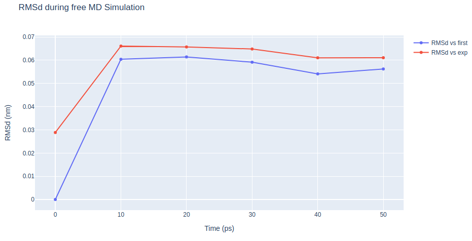
Step 3: Checking free MD simulation results

Checking results for the final step of the setup process, the free MD run. Plotting Root Mean Square deviation (RMSd) and Radius of Gyration (Rgyr) by time during the free MD run step. RMSd against the experimental structure (input structure of the pipeline) and against the minimized and equilibrated structure (output structure of the NPT equilibration step).

# GMXRms: Computing Root Mean Square deviation to analyse structural stability 
#         RMSd against minimized and equilibrated snapshot (backbone atoms)   

from biobb_analysis.gromacs.gmx_rms import gmx_rms

# Create prop dict and inputs/outputs
output_rms_first = pdbCode+'_'+ligandCode+'_rms_first.xvg'
prop = {
    'selection':  'Backbone'
}

# Create and launch bb
gmx_rms(input_structure_path=output_gppmd_tpr,
         input_traj_path=output_md_trr,
         output_xvg_path=output_rms_first, 
          properties=prop)

# GMXRms: Computing Root Mean Square deviation to analyse structural stability 
#         RMSd against experimental structure (backbone atoms)   

from biobb_analysis.gromacs.gmx_rms import gmx_rms

# Create prop dict and inputs/outputs
output_rms_exp = pdbCode+'_'+ligandCode+'_rms_exp.xvg'
prop = {
    'selection':  'Backbone'
}

# Create and launch bb
gmx_rms(input_structure_path=output_gppmin_tpr,
         input_traj_path=output_md_trr,
         output_xvg_path=output_rms_exp, 
          properties=prop)

import plotly
import plotly.graph_objs as go

# Read RMS vs first snapshot data from file 
with open(output_rms_first,'r') as rms_first_file:
    x,y = map(
        list,
        zip(*[
            (float(line.split()[0]),float(line.split()[1]))
            for line in rms_first_file 
            if not line.startswith(("#","@")) 
        ])
    )

# Read RMS vs experimental structure data from file 
with open(output_rms_exp,'r') as rms_exp_file:
    x2,y2 = map(
        list,
        zip(*[
            (float(line.split()[0]),float(line.split()[1]))
            for line in rms_exp_file
            if not line.startswith(("#","@")) 
        ])
    )
    
trace1 = go.Scatter(
    x = x,
    y = y,
    name = 'RMSd vs first'
)

trace2 = go.Scatter(
    x = x,
    y = y2,
    name = 'RMSd vs exp'
)

data = [trace1, trace2]

plotly.offline.init_notebook_mode(connected=True)

fig = ({
    "data": data,
    "layout": go.Layout(title="RMSd during free MD Simulation",
                        xaxis=dict(title = "Time (ps)"),
                        yaxis=dict(title = "RMSd (nm)")
                       )
})

plotly.offline.iplot(fig)

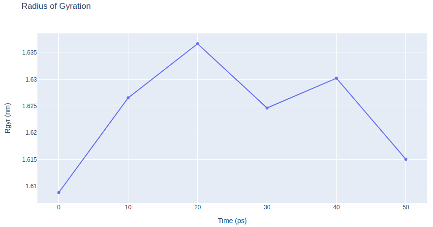
# GMXRgyr: Computing Radius of Gyration to measure the protein compactness during the free MD simulation 

from biobb_analysis.gromacs.gmx_rgyr import gmx_rgyr

# Create prop dict and inputs/outputs
output_rgyr = pdbCode+'_'+ligandCode+'_rgyr.xvg'
prop = {
    'selection':  'Backbone'
}

# Create and launch bb
gmx_rgyr(input_structure_path=output_gppmin_tpr,
         input_traj_path=output_md_trr,
         output_xvg_path=output_rgyr, 
          properties=prop)

import plotly
import plotly.graph_objs as go

# Read Rgyr data from file 
with open(output_rgyr,'r') as rgyr_file:
    x,y = map(
        list,
        zip(*[
            (float(line.split()[0]),float(line.split()[1]))
            for line in rgyr_file 
            if not line.startswith(("#","@")) 
        ])
    )

plotly.offline.init_notebook_mode(connected=True)

fig = ({
    "data": [go.Scatter(x=x, y=y)],
    "layout": go.Layout(title="Radius of Gyration",
                        xaxis=dict(title = "Time (ps)"),
                        yaxis=dict(title = "Rgyr (nm)")
                       )
})

plotly.offline.iplot(fig)

Post-processing and Visualizing resulting 3D trajectory

Post-processing and Visualizing the protein-ligand complex system MD setup resulting trajectory using NGL

Step 1: Imaging the resulting trajectory, stripping out water molecules and ions and correcting periodicity issues.
Step 2: Generating a dry structure, removing water molecules and ions from the final snapshot of the MD setup pipeline.
Step 3: Visualizing the imaged trajectory using the dry structure as a topology.

Building Blocks used:

GMXImage from biobb_analysis.gromacs.gmx_image
GMXTrjConvStr from biobb_analysis.gromacs.gmx_trjconv_str

Step 1: Imaging the resulting trajectory.

Stripping out water molecules and ions and correcting periodicity issues

# GMXImage: "Imaging" the resulting trajectory
#           Removing water molecules and ions from the resulting structure
from biobb_analysis.gromacs.gmx_image import gmx_image

# Create prop dict and inputs/outputs
output_imaged_traj = pdbCode+'_imaged_traj.trr'
prop = {
    'center_selection':  'Protein_Other',
    'output_selection': 'Protein_Other',
    'pbc' : 'mol',
    'center' : True
}

# Create and launch bb
gmx_image(input_traj_path=output_md_trr,
         input_top_path=output_gppmd_tpr,
         input_index_path=output_complex_ndx,
         output_traj_path=output_imaged_traj, 
          properties=prop)

Step 2: Generating the output dry structure.

Removing water molecules and ions from the resulting structure

# GMXTrjConvStr: Converting and/or manipulating a structure
#                Removing water molecules and ions from the resulting structure
#                The "dry" structure will be used as a topology to visualize 
#                the "imaged dry" trajectory generated in the previous step.
from biobb_analysis.gromacs.gmx_trjconv_str import gmx_trjconv_str

# Create prop dict and inputs/outputs
output_dry_gro = pdbCode+'_md_dry.gro'
prop = {
    'selection':  'Protein_Other'
}

# Create and launch bb
gmx_trjconv_str(input_structure_path=output_md_gro,
                input_top_path=output_gppmd_tpr,
                input_index_path=output_complex_ndx,
                output_str_path=output_dry_gro, 
                properties=prop)

Step 3: Visualizing the generated dehydrated trajectory.

Using the imaged trajectory (output of the Post-processing step 1) with the dry structure (output of the Post-processing step 2) as a topology.

# Show trajectory
view = nglview.show_simpletraj(nglview.SimpletrajTrajectory(output_imaged_traj, output_dry_gro), gui=True)
view

Output files

Important Output files generated:

3HTB_JZ4_md.gro: Final structure (snapshot) of the MD setup protocol.
3HTB_JZ4_md.trr: Final trajectory of the MD setup protocol.
3HTB_JZ4_md.cpt: Final checkpoint file, with information about the state of the simulation. It can be used to restart or continue a MD simulation.
3HTB_JZ4_gppmd.tpr: Final tpr file, GROMACS portable binary run input file. This file contains the starting structure of the MD setup free MD simulation step, together with the molecular topology and all the simulation parameters. It can be used to extend the simulation.
3HTB_JZ4_genion_top.zip: Final topology of the MD system. It is a compressed zip file including a topology file (.top) and a set of auxiliary include topology files (.itp).

Analysis (MD setup check) output files generated:

3HTB_JZ4_rms_first.xvg: Root Mean Square deviation (RMSd) against minimized and equilibrated structure of the final free MD run step.
3HTB_JZ4_rms_exp.xvg: Root Mean Square deviation (RMSd) against experimental structure of the final free MD run step.
3HTB_JZ4_rgyr.xvg: Radius of Gyration of the final free MD run step of the setup pipeline.

Questions & Comments

Questions, issues, suggestions and comments are really welcome!

GitHub issues:
- https://github.com/bioexcel/biobb
BioExcel forum:
- https://ask.bioexcel.eu/c/BioExcel-Building-Blocks-library

Protein Ligand Complex MD Setup tutorial using BioExcel Building Blocks (biobb)

Settings

Biobb modules used

Auxiliary libraries used

Conda Installation and Launch

Pipeline steps:

Input parameters

Fetching PDB structure

Visualizing 3D structures

Fix protein structure

Create protein system topology

Create ligand system topology

Step 1: Add hydrogen atoms

Step 2: Energetically minimize the system with the new hydrogen atoms.

Visualizing 3D structures

Preparing Ligand Restraints

Step 1: Creating an index file for the small molecule heavy atoms

Step 2: Generating the position restraints file

Create new protein-ligand complex structure file

Create new protein-ligand complex topology file

Create solvent box

Fill the box with water molecules

Visualizing 3D structure

Adding ions

Step 1: Creating portable binary run file for ion generation

Step 2: Adding ions to neutralize the system and reach a 0.05 molar concentration

Visualizing 3D structure

Energetically minimize the system

Step 1: Creating portable binary run file for energy minimization

Step 2: Running Energy Minimization

Step 3: Checking Energy Minimization results

Equilibrate the system (NVT)

Step 1: Creating an index file with a new group including the protein-ligand complex

Step 2: Creating portable binary run file for system equilibration (NVT)

Step 3: Running NVT equilibration

Step 4: Checking NVT Equilibration results

Equilibrate the system (NPT)

Step 1: Creating portable binary run file for system equilibration (NPT)

Step 2: Running NPT equilibration

Step 3: Checking NPT Equilibration results

Free Molecular Dynamics Simulation

Step 1: Creating portable binary run file to run a free MD simulation

Step 2: Running short free MD simulation

Step 3: Checking free MD simulation results

Post-processing and Visualizing resulting 3D trajectory

Step 1: Imaging the resulting trajectory.

Step 2: Generating the output dry structure.

Step 3: Visualizing the generated dehydrated trajectory.

Output files

Questions & Comments